This is the first article in a series on Uniswap v3 liquidity provision (LP) strategies. The goal of the series is to help readers better understand LP on Uniswap v3, and discuss some ways to protect their investments.

A Motivating Example
On March 11, 2023, Uniswap had its maximum transaction volume so far: nearly 12 billion USD. This spike in the on-chain trading volume was largely caused by fluctuations in USDC and other stablecoin prices.
For context, Uniswap’s volume was almost two thirds of the largest CEX (Binance’s) volume on the same day.
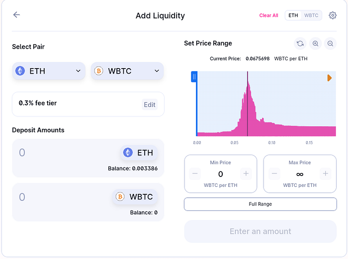
If you had put a single ETH in the Uniswap’s USDC/WETH 0.05% pool at the start of 11th March, selecting the reasonable price range from 1450 to 1700 USDC per ETH, your position would have received 0.026 ETH in fees in the following 24 hours (according to Uniswap subgraph data). This corresponds to an astonishing 953% fee APR. As the initial price of ETH in terms of USDC was slightly below 1450 USDC/ETH, that would have been a single-sided liquidity position at the start. At the end, both assets would have been in the pool, with the final value of assets roughly equal to 0.99 ETH. The total return on the investment, including this loss, still would have been more than 550% APR.

The returns on an average trading day are not nearly as extreme as the outlier of 11th March. Nonetheless, some DeFi tools report that Arbitrum’s USDC/WETH pool’s average yield (30 day APY) is 98.71%, and it remains in the double digits even on slow days. So, why isn’t the whole crypto world putting their ETH in Uniswap v3? The answer, of course, is related to the risks that Uniswap LPs take on.

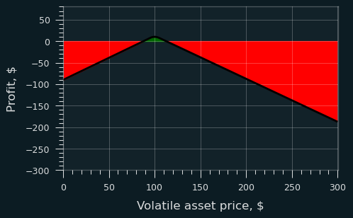
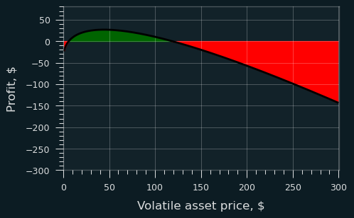
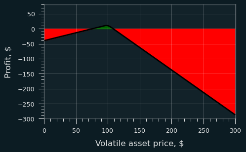
One issue is illustrated in the figure above: narrow-range positions tend to have limited upside potential, but unlimited downside risks. It may be a good idea to hedge the position in order to protect your investment.

Why this article?
Uniswap v3 is a complex protocol, and very different from the previous version, Uniswap v2. The main novelty in v3 is the concentrated liquidity (CL) feature, which allows the liquidity providers specify a price range in which their capital is active. CL decreases the price impact of trades and in this way lets the traders to get a better user experience.
I have been Uniswap v3 user and consultant for almost two years, and have written a popular explainer on the v3 math. In this role, I have talked with quite a few people interested in becoming Uniswap v3 LPs, and seen some typical gaps in knowledge and understanding. I have also seen some typical LP strategies emerging, sometimes being independently re-invented, and the drawbacks and tradeoff being unclear. This series of articles aims to improve the state of the knowledge in the community. This first article is an overview at a higher level of abstraction, but bear with me, there will be follow-up articles with more concrete discussions or even walkthroughs.
Even if you’re marginally interested in Uniswap, understanding the costs and tradeoffs of Uniswap v3 LP may be a good idea. One reason is that Uniswap v3 is a systemically important protocol for DeFi. After all, liquidity providers (LP), while motivated by selfish profits, provide a very important service to the whole crypto ecosystem. Deep liquidity in DEX pools is important for everyone on DeFi; this is the only way how decentralized alternatives can hope to compete with custodial and permissioned exchanges.
Another reason is that there is a growing ecosystem of protocols connected to Uniswap or inspired by Uniswap v3: an ecosystem that may even be named DeFi 3.0 one day. Ideas such as concentrated liquidity (CL), avoiding external oracles, mixing order-book AMM principles, allowing the users fine-grained control over liquidity allocation strategies, option-like payoffs etc. have found their way in protocols such as Panoptic, Infinity Pools, Smilee Finance, Numoen, Ajna Finance (for oracle-free lending), Gamma Swap and others. Management and autocompounding protocols such as Arrakis Finance also should be noted. Some of these protocols are going to offer new hedging opportunities or new income sources for the LPs; to understand the potential of these new protocols, it may be a good idea to start with understanding the risks and rewards of the current Uniswap LPs.
What is your benchmark?
A benchmark is a standard against which something is compared. The benchmark that you personally should select depends on your goals as a LP. Here are some DeFi-native benchmarks that can serve as alternatives for Uniswap LP positions:
- composite positions of stable and volatile assets, such as the 50:50 HODL;
- holding only the volatile asset;
- holding only the stable asset;
- advanced strategies such as rebalancing (buying and selling assets to reach a specific balance in your portfolio), just-in-time LP, running arbitrage bots and so on. These strategies, by definition, are not available to most on-chain market participants.
Furthermore, all assets that are not in LP positions can earn lending fees or staking yields. Aave and Curve pools, as well as ETH staking, can provide the “risk-free” DeFi benchmark rate.
The 50:50 HODL benchmark is traditional in the community and will be the focus of this article (named simply as HODL). However, it’s important to realize that it’s not the only available benchmark. For instance, for delta-neutral strategies a better benchmark is the “risk-free” rate on stablecoins.
The profit and loss (PnL) of a Uniswap LP depends on liquidity concentration levels. At one extreme, Uniswap v3 LPs can simulate v2 behavior by selecting a full-range position. (Using full range positions in v3 may be a viable LP strategy as well: see this article from Uniswap Labs for in-depth treatment.) At the other extreme, liquidity can be concentrated in a narrow price range. A CL position earns high fees when in range, but for volatile assets, it is mathematically expected to leave the range rapidly.
Once again, when evaluating a selected LP strategy, you should be clear about your own goals, pick a suitable benchmark to play the role of a “reasonably good” investment for you, and use that to compare the expected PnL of other strategies. To better understand this point, let’s ask the question “What is a good investment?” in the TradFi context. Is it the 1% APR that a bank offers on a “high-yield” saving account? The 3% APR government bonds? The 5–10% annual growth of solid ETFs? Is it just storing cash, and waiting to the market to crash? Or is it the profits of your “smarter” friend who likes to pick stocks, and claims to have tripled his investment in the 2021 alone, but stopped talking about his portfolio in 2022? Probably all of them, to some extent — the Pareto-efficient frontier in the risk/reward space almost surely consists of mixed-asset portfolios. In any case, it’s easy to beat not just the expected value of something like 1% savings account, but also its Sharpe ratio (in other words, the risk-adjusted reward is higher as well). The expected value of some other portfolios will be much harder to beat; to do that you’d need to take on more risk. And it’s not just the risk, your beliefs about the expected price action also play a role in selecting the benchmark.
Formalizing some benchmarks
(Feel free to skip this section if you’re not interested in the math!)
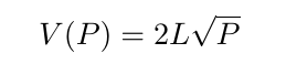
The value of a LP position is:

where the price P is defined simply as P := y/x.
Let’s assume a “standard” constant product automated market maker (AMM). The relation between the amounts of assets in a position is defined with the function x·y=k, where k is a constant. The pool’s liquidity L is defined such that L² := k. With a bit of algebra it follows that:
If the price P changes, then V(P) also changes. Let’s denote the price at moment T with P_T, the value with V_T, and the ratio of prices P_T/P_0 with α. Then:
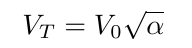
In other words, the value function of LP position is a square root function.
Following the Black-Scholes model, let us use Δ (delta) to denote the price-dependence of the value function, and Γ (gamma) to denote the price-dependence of the delta. These are the first and second derivatives of the LP position’s value function, with respect to price:

Given the value function as above, these derivatives are:

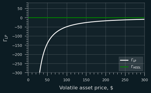
The gamma term is a non-linear, always negative function that describes the so-called impermanent loss of a LP position. (See these references for an in-depth treatment of the subject.) In contrast, 50:50 HODL and 100% asset holdings have zero gamma, so no impermanent loss:
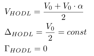
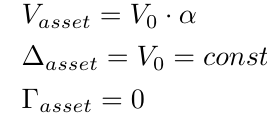
When normalized against the initial value V_0, 50:50 HODL position’s delta is 0.5, and asset’s position’s delta is 1.0, as expected.
Another way to think about the LP position:
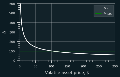
- if the asset price increases, then LP’s delta is lower than the delta of a 50:50 HODL position;
- if the asset price decreases, then LP’s delta is higher.
The LP position is underexposed to price increases, and overexposed to price decreases. When price goes up, the gain of the LP is reduced; when the price goes down, their loses increased.
This is not a problem specific to the Uniswap. LP gamma is expected to be negative in all reasonable AMMs, as shown in the LVR paper and in other research.
The math for the narrow-range positions (concentrated liquidity) is a fair bit more complex¹. Nevertheless, the primary intuition you should have about concentrated liquidity is that it makes all things more extreme. Fee income is amplified while the position is in range, but impermanent loss is amplified as well. Another important ideas is that CL introduces new risks (going out of range) as well as opportunities (range orders, limit orders).
¹ —The derivation of delta and gamma for CL positions is left as an exercise to the reader. The v3 whitepaper and my explainer can be a good starting point.
PnL of unprotected LP positions
Let’s take a step back and ask yourself: do I really want to exposed to something that changes in value with the square root of price?
In some cases, the answer may be “yes, as a form of rebalancing”. Nevertheless, for the vast majority of DeFi participants, the square-root function is an arbitrary and weird thing which to maximize. Almost certainly there’s a better risk-reward function for your risk tolerance levels.

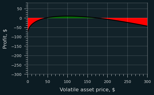
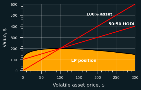
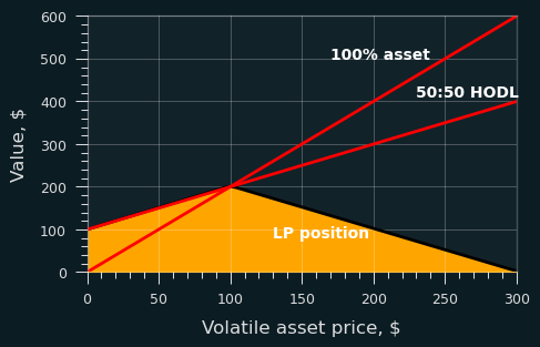
For the figures I’m modeling a liquidity pool with one volatile and one stable asset, the initial price of the volatile asset $100, the initial value of the pool $200.
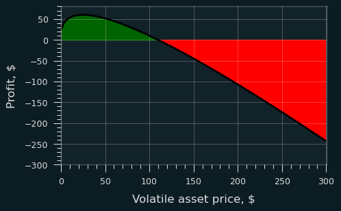
The figure above shows the shape of the LP value function relative to the benchmarks. The figure below shows the profit relative to HODL. The LP position is assumed to collect 5% of its initial value in fees: a simplification that is not fully realistic, but gives something to start with.
Even under this assumption of the relatively high 5% fees, the LP suffers losses if the price changes significantly enough.
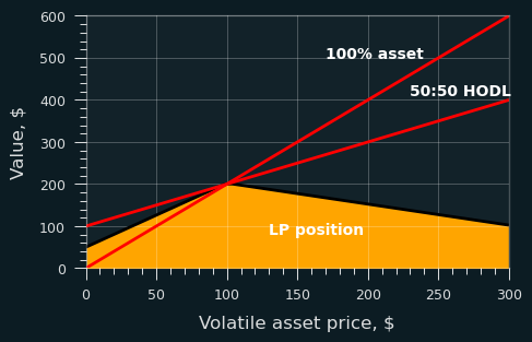
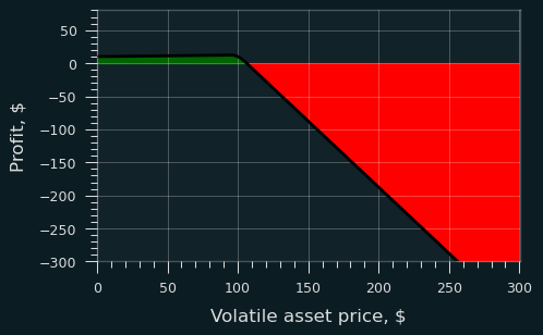
The situation for v3 concentrated liquidity positions is way more dramatic:

The LP’s potential reward in this scenario appears to be significantly outweighed by the risk, as they may end up with a small green island in a sea of red, making it a very high-risk proposition if left unmanaged. While the fees earned by the concentrated liquidity positions can be much higher than those of v2-style full range positions, these fees are only accrued when the price is in the position’s range, meaning that losses due to large price volatility is unlikely to be fully compensated with matching increase in LP fees.
Hedging using borrowed funds
As shown above, entering into unprotected LP positions, especially those with a narrow range, can be a high-risk strategy and may often be unprofitable.
A LP position can be hedged by putting in more funds as a collateral, and borrowing the volatile asset. 100% or less of the volatile asset can be borrowed (the rest owned), depending on the position’s desired value function and payoff function.
A related idea is to short-sell the volatile asset via margin-trading. Here I prefer the borrowing approach because its a DeFi-native strategy. However, it is a more capital-intensive approach, because DeFi only supports overcollateralized loans, while short-selling can be done on a margin, and dot nor require as much initial capital. On the other hand, under normal market conditions, overcollateralized borrowing is likely to have a positive net APR, while the funding rate for margin trading likely to be negative. Finally, liquidation risks are unfortunately present in both strategies.
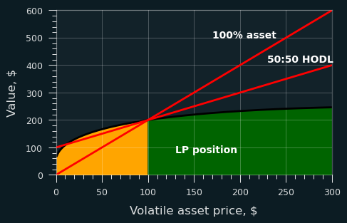
As shown in the figures above, for full-range LP positions using borrowed assets reduces the downside risk when price goes down, and the cost of increasing the downside risk when the price goes up.
For narrow-range positions, the downside risk on price decrease can be perfectly hedged, when 100% of the volatile asset is borrowed. Compared with just holding stablecoins, the PnL would still be negative, however. To match the PnL of stablecoins, one would need to borrow 200% of the volatile asset initially required for the pool, and short-sell the half left over after initializing the LP position.
There is a symmetrical strategy that aims to protect the gains in case the asset price goes up. In other words, this is a strategy to use if you’re bullish on the volatile asset. Instead of borrowing the asset or shorting it, you’d either buy the asset and borrow stablecoins against it, or long it on a margin. The payoffs are symmetrical to the ones discussed above, just the x-axis inverted.
Summary of payoffs
The table below shows the PnL of various positions relative to the 50:50 HODL position, under decreasing️️ 📉, mean-reverting️, and increasing️ 📈prices. “Cash” means a position in fiat or stablecoins.
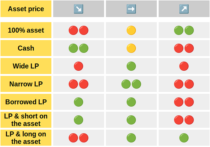
A few caveats:
- this is to get rough intuition only, for accurate results you’d need to be very clear about your assumptions and model the positions mathematically;
- as discussed above, 50:50 HODL isn’t always the benchmark you’d want to use;
- “Borrowed LP” and “LP & short on the asset” strategies are shown separately for clarity, even though the payoffs are almost identical, as discussed above.
Conclusion
To summarize:
- Uniswap pools offer a real yield opportunity and are systemically important for DeFi.
- Entering unprotected LP positions, especially narrow-range positions, is rarely a good strategy.
- Downside risks can be hedged by using borrowed funds, or by short-selling the volatile asset.
This article is the first in a series about Uniswap LP strategies. More precise hedging of LP position is possible with advanced techniques, such as power perpetuals and options. These will covered in the next articles, along with other topics such as strategic liquidity relocation (position rebalancing). Follow me on Twitter to get faster updates!
Acknowledgements. This work received financial support from the Uniswap Foundation. Thanks for comments on a draft version from Fedeebasta.eth, Alain from Newbridge, Nikos Baxevanis and Antonios Klimis.
Disclaimer. This post is for general information purposes only. It does not constitute investment advice or a recommendation or solicitation to buy or sell any investment and should not be used in the evaluation of the merits of making any investment decision. It should not be relied upon for accounting, legal or tax advice or investment recommendations. This article was written in the author’s free time and is not related to his professional activity or his employer. This post reflects the current opinions of the author, which are subject to change without being updated.